Network Abstraction and Virtualization: Where to Start?
With the growth of server virtualization network designs and the associated network management constructs have been stretched beyond their intended uses. This has brought about data center networks that are unmanageable and slow to adapt to change. While servers and storage can be rapidly provisioned to bring on new services the network itself has become a bottleneck of required administrative changes and inflexible constructs limiting scalability and speed of adoption.
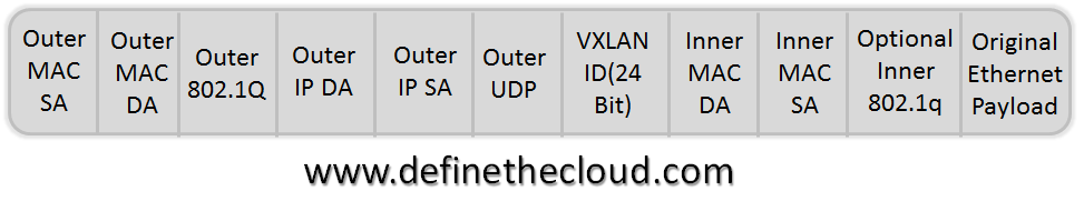
These constraints of modern data center networks have motivated network architects to look for workarounds of which one current proposal is ‘network virtualization’ which looks to apply the benefits of server virtualization to the network. Conceptually network virtualization is the use of encapsulation techniques to create virtual overlays on existing network infrastructure. These methods use technologies such as VxLAN, STT, NVGRE, and others to wrap machine traffic in virtual IP overlays which can be transported across any Layer 3 infrastructure.
1. A primary benefit of these overlay techniques is the ability to scale beyond the limits of VLANs for network segmentation. Virtualization and multi-tenancy caused an explosion of network segments that strain traditional isolation techniques. With VLANs we are limited at 4096 segments or less depending on implementation. Other methods exist, such as placing ACLs within the Hypervisor but these also suffer limits in configuration and CPU overhead. The purpose of these techniques is creating application/tenant segmentation without security implications between segments. As the number of services and tenants grows these limits quickly become restrictive.
2. Another advantage of the network virtualization overlay is the ability to place workloads independent of physical locality and underlying topology. As long as IP connectivity is available the encapsulation handles delivery to end-point workloads. This provides greater flexibility in deployment, especially for virtualized workloads which receive encapsulation within the hypervisor switch. The operational benefit of this effect is the ability to place workloads where there is available capacity without restrictions from underlying network constructs.
Network virtualization does not come without drawbacks. The act of layering virtual networks over existing infrastructure puts an opaque barrier between the virtual workloads and the operation of the underlying infrastructure. This brings on issues with performance, quality of service (QoS) and network troubleshooting. Unlike server virtualization this limitation is not seen with compute hypervisors which are tightly coupled with the hardware maintaining visibility at both levels. The diagram below shows the relationship between network and server virtualization.

1. This lack of cross-visibility between the logical networks carrying production application traffic, and the physical network providing the packet delivery, leads to issues with application performance and system troubleshooting. With SDN techniques based on network virtualization through encapsulation, the packet delivery infrastructure is completely obfuscated by the encapsulation. This can lead to performance issues arising from lack of quality of service, altered multi-pathing ability, and others within the underlying network. This separation is shown in the diagram below.

2. Additionally these logical networks add a point of management to the network architecture. While they can hide the complexity of the underlying network for the purposes of application deployment, the network underneath still exists. The switching infrastructure must still be configured, managed and deployed as usual. All of the constructs shown above must still be architected and pushed into device configuration. Network virtualization provides perceived independence from the infrastructure but does not provide a means to manage the network as a whole.
3. The last challenge for network virtualization techniques is the ability to tie overlays back to traditional networking constructs understood by the network switches below. Switch hardware and software is designed to use VLANs which are tied to IP subnets and stitch security and services to these constructs. The overlay created by encapsulation does not alleviate these issues.
For example encapsulation techniques such as VxLAN provide far greater logical network scalability upwards of 16 million virtual networks. This logical scalability does not currently stitch into traditional switching equipment that assumes VLANs are global. Tighter cohesion will be required between physical switching infrastructure and hypervisor based access layers to provide robust services to real-world heterogeneous environments.
While overlay techniques provide separate namespace and therefore a means for overlapping IP addressing there will still be a need to architect the routing that handles this. In order to accomplish this network functionality such as Virtual Routing and Forwarding (VRF) must be configured on the switching infrastructure, or virtual routers deployed in the hypervisor. VRF scalability is greatly limited by hardware implementation and will be far less than VxLAN scalability, while virtualized routers will consume CPU overhead and require additional architectural considerations. Without techniques in place network tenants will require non-overlapping IP space.
Making a case for true abstraction
With network virtualization alone being overlaid onto existing infrastructure we just add layers of complexity. This occurs without correcting the issues that have arisen in traditional networking constructs; just adding network virtualization will do no more than amplify existing problems. A parallel can be drawn to server virtualization where the more rapid pace of server provisioning quickly brought out problems in underlying architecture and processes.
The underlying network consists of hardware, cabling, and Layer 2 / Layer 3 topologies that dictate traffic flow and potential application throughput. These layers have their own limitations and stability issues which are not addressed by network virtualization. Think of the OSI model in terms of building a house, the bottom layers (1-3) create a foundation, a frame, and a structure. Issues in those foundational layers will be exacerbated at each additional layer added on top.
Rather than applying an overlay technique such as a virtualization layer on top of existing architecture, IT architects will benefit greatly from abstracting the network constructs from the ground up first. Separating out logical and physical constructs, security, services, etc. prior to layering on overlays will provide a clean canvas on which to paint the future’s scalable feature rich networks. Virtualization must be built into the network from the ground up rather than layered on top. Again this parallels server virtualization where the greatest success has been seen in full virtualization of the hardware platform and tight integration down to bare metal. The end goal is addressing the underlying network issues rather than mask them with a virtualization layer.
The ties between network constructs such as VLAN, IP subnet, security, load-balancing etc. have placed constraints on the scalability and agility of the network. Each VLAN is provided an IP subnet, security and network services are then tied to these constructs. Addressing and location become the identifying characteristics of the network rather than the application requirements. This is not optimal behavior for a network responsible for elastic business services, workload anywhere designs, and ever increasing connectivity needs. These attributes and capabilities of connectivity must be abstracted in a new way to allow us to move beyond the constraints we have imposed by overloading or misusing these basic network constructs.
 Rather than starting with a new coat of paint on a peeling building, abstraction takes a ground up approach. By looking at the purpose of each construct: VLAN = Broadcast domain, IP = addressing mechanism, etc. we can redesign with a goal to alleviate the unnecessary constraints that have been placed on today’s networks. With these constructs separated we can provide a transport capable of maximizing the performance, security and scalability of the applications using it.
Take a step back from traditional network thinking and think in terms of application needs without consideration of current deployment methodology. Think through the following questions leaving out concepts like: VLAN, Subnet, IP addressing, etc.:
- How would you tie application tiers together?
- How would you group like services?
- What policies would be required between application tiers?
- What services are required for a given application?
- How does that application connect to the intranet and internet?
Separating out the applications and services required from the underlying architecture is not possible with today’s networks, virtualized or not. Overlay network virtualization alone may hide some of the complexities but does not provide tools for optimizing the delivery and holistic design. The conversation must include addressing, VLAN construct, location and service insertion. If these constructs are instead abstracted from one another, and the architecture, the conversation can revolve around application requirements rather than network restrictions.
Summary:
While network virtualization provides a set of tools for gaining greater network scale and application deployment flexibility, it is not a complete solution. Without true network abstraction and tools for visibility between the logical and physical network virtualization does no more than add complexity to existing problems. As was seen with server virtualization, layering virtualization on infrastructure issues and bad processes exponentially increases the complexity and room for error.
In order to truly scale networks in a sustainably manageable fashion we need to remove the ties of disparate network constructs by abstracting them out. Once these constructs operate independently of one another we’re provided a flexible architecture that removes the inherent complexity rather than leaving the problems and compounding them through layers of virtualization.
To build networks that meet current demands while being able to support the rapid scale and emerging requirements we need to rethink network design as a whole. Taking a top down look at what we need from the network without tying ourselves to the way in which we use the constructs today allows us to design towards the future and apply layers of abstraction down the stack to meet those goals.
Thinking about your network today, is virtualization alone solving the problems or adding a layer?
Network virtualization without network abstraction – results in short term patching with limited control of longer term operational complexity.
Network virtualization based on an abstracted network – results in effective control of both capital and operational expenses.